CorrelationSimilarity
This metric measures the correlation between a pair of numerical columns and computes the similarity between the real and synthetic data -- aka it compares the trends of 2D distributions. This metric supports both the Pearson and Spearman's rank coefficients to measure correlation.
Data Compatibility
Numerical : This metric is meant for continuous, numerical data
Datetime : This metric converts datetime values into numerical values
This metric ignores missing values.
Score
(best) 1.0: The pairwise correlations of the real and synthetic data are exactly the same
(worst) 0.0: The pairwise correlations are as different as they can possibly be
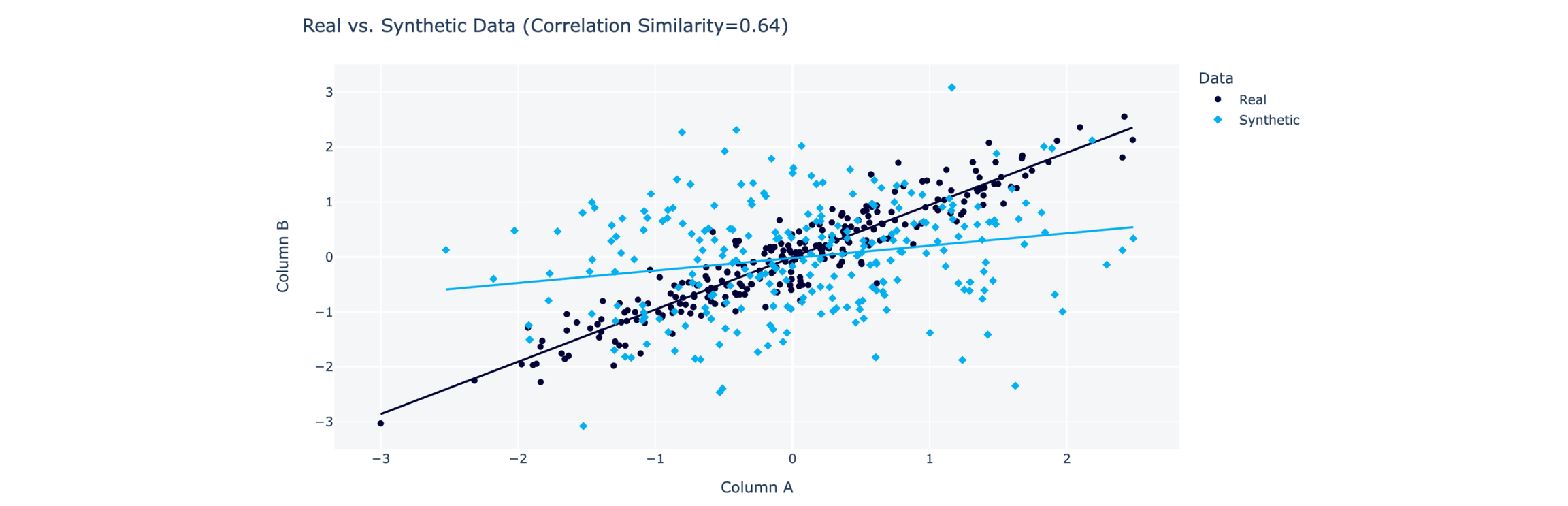
Below is a graph that shows some fictitious data for 2 columns of real and synthetic data (black and blue, respectively). The Correlation Similarity Score is 0.64.
How does it work?
For a pair of columns, A and B, this test computes a correlation coefficient on the real and synthetic data, R and S. This yields two separate correlation values. The test normalizes and returns a similarity score using the formula below.
Note that there are multiple ways to compute the correlation coefficient. This supports both the Pearson correlation coefficient [1][2] and the Spearman's rank correlation coefficient [3][4]. Both are bounded between -1 and +1.
Pearson vs. Spearman Coefficients
The Pearson and Spearman rank correlation coefficients are commonly used in data science applications. The Pearson coefficient measures whether two columns are linearly correlated while the Spearman measures whether they are monotonically related.
Both coefficients range from -1 to +1. A rough interpretation is given in the table below.
| Score | Pearson Coefficient | Spearman's Rank Coefficient |
|---|---|---|
+1 | As one column increases, the other increases linearly | As one column increases, the other increases too |
0 | As one column increases, the other column has no linear pattern | As one column increases, the other column has no pattern |
-1 | As one column increases, the other decreases linearly | As one column increases, the other decreases too |
Usage
Recommended Usage: The Quality Report applies this metric to every pair of compatible columns and provides visualizations to understand the score.
To manually run this metric, access the column_pairs module and use the compute method.
Parameters
(required)
real_data: A pandas.DataFrame object containing 2 columns of real data(required)
synthetic_data: A pandas.DataFrame object containing 2 columns of synthetic datacoefficient: A string that describes the correlation coefficient to use:(default)
'Pearson'for the Pearson correlation coefficient [1]'Spearman'for the Spearman's rank correlation coefficient [3]
FAQs
Technical Note: What is captured by this metric?
The correlation describes whether the data closely follows a trend or whether it's noisy. The CorrelationSimilarity score describes whether the correlations of the real and synthetic data are similar.
Be careful when interpreting this metric, as some scenarios are not easily apparent.
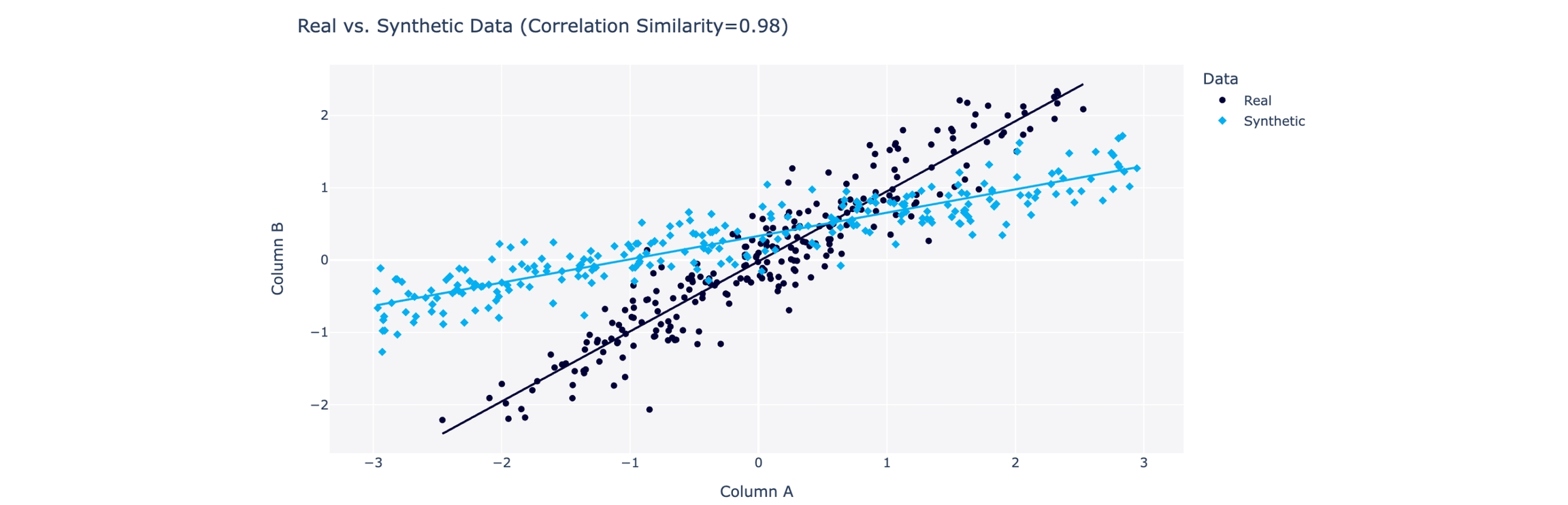
Correlation does not describe any details about the trend, such as the slope of a line or its overall shape. For example, the data below has a near perfect score of 0.98 because both the real and synthetic data have strongly positive linear correlations. However, the slopes of the lines are different.
The CorrelationSimilarity score can be high if your data is noisy. If both the real and synthetic data don't have any clear trends, the correlation for both will be around 0. In this case, you will see a high CorrelationSimilarity score, indicating that the the synthetic data is successfully capturing the non-existent "trend".
References
[1] https://en.wikipedia.org/wiki/Pearson_correlation_coefficient
[2] https://docs.scipy.org/doc/scipy/reference/generated/scipy.stats.pearsonr.html
[3] https://en.wikipedia.org/wiki/Spearman%27s_rank_correlation_coefficient
[4] https://docs.scipy.org/doc/scipy/reference/generated/scipy.stats.spearmanr.html
Last updated